Gradient removal with Pixinsight

Astrophotographers are well aware of the effects of light pollution due to light from cities or the Moon on their images, producing differences in the brightness of the sky background depending on the areas of the sky. the image we call gradients. There are different forms of gradients, more or less complex to process, depending on their origin (Moon, streetlights, vignetting not corrected by flats, etc.) and their intensity.

Fortunately, modern astronomical image processing software has a gradient removal tool. and the one featured here from Pixinsight software is absolutely fantastic.

While it is obvious that getting out of cities, or even climbing to the top of mountains is ideal for any astrophotographer, it is not always possible and for those like me who have chosen to image in a fixed position in the city. rather than nomadic, it will be necessary to deal with the loss of detectivity due to light pollution (the weakest signals being irremediably drowned in it) and the gradients which can be processed in software.

Pixinsight has two gradient removal processes: AutomaticBackgroundExtractor and DynamicBackgroundExtraction.

The removal of gradients is a painstaking process that in most cases cannot be done automatically without operator intervention. However, in the simplest cases the automatic Pixinsight gradient extraction process may prove to be sufficient, and otherwise the dynamic gradient extraction process will be formidable to overcome more complex gradients.

The purpose of this article will be to describe in detail the operation of these two processes, in order to better understand them and thus better choose them according to the image to be processed, and potentially better use them.

We will first review in detail the different parameters of these two processes and their functions, then we will apply them to concrete cases on images.

Do not worry the functions and parameters are very numerous but in practice we only use a small part. However, it is useful to understand these parameters in order to understand why they are used or not, and what they can possibly be used for to better understand the operation of the process.

A very basic and fast use is possible with the two processes by not modifying or modifying the basic settings very little. Adjusting these parameters can be useful in some cases of complex gradients, or to save time in creating the sky background samples.

Obviously and as always, let us remember that there is no one way to proceed that would be the one and only truth. Also the approach and the method proposed here are the fruit of my experience of urban astrophotography and cannot be claimed to be universal and incontestable.

To continue

DESCRIPTION OF AUTOMATIC BACKGROUND EXTRACTOR

To continue

USE OF AUTOMATIC BACKGROUND EXTRACTOR

To continue

DESCRIPTION OF DYNAMIC BACKGROUND EXTRACTION

To continue

USING DYNAMIC BACKGROUND EXTRACTION

To continue

Case of automatic placement of samples (galaxy, cluster etc ...)

To continue

Case of manual placement of samples (large nebulae, presence of IFN etc ...)

To continue

OTHER EXAMPLES OF COMPLEX GRADIENT WITHDRAWALS

Ancre 1

DESCRIPTION OF AUTOMATIC BACKGROUND EXTRACTOR

As the name suggests, ABE works fully automatically: you provide a source image, a number of parameters controlling ABE's behavior, and you get another image with the generated background template.

This model can be applied to the original image by subtraction or division, depending on the type of uneven illumination problems to be corrected.

Additive phenomena like light pollution gradients must be corrected by subtraction, while multiplicative effects like vignetting must be corrected by division (although in this case correct calibration of the image by acquiring flats is necessary. the appropriate procedure) .

One of the possibilities offered by ABE is to apply it in batch on raw images before alignment and stacking, which makes it possible to process the images individually and in an automated way in order to avoid the complex combination of gradients (stacking). that can change from one raw to another over the same night or several nights (position of the object in the sky in relation to the light pollution halo, position of the Moon, etc.).

In practice, this could be useful if we are sure that the raw images are only affected by a simple gradient that can be processed by ABE without risk of alteration of the signal. For more caution it is still preferable to have control over the gradient extraction and therefore to perform it on the final stack, because it would be laborious to apply it manually on each raw material, especially since the RSB of a unitary pose does not always make it possible to distinguish the gradients.

Personally I use very little ABE because even if it can give the impression of a satisfactory result nothing can replace the control offered by DBE, whether on rather simple fields offering a lot of sky background areas as on the more complex field of nebulosities covering the field. It must also be said that when imagining in the city I have more often to do with complex gradients.

Let us first see the description of the various ABE parameters (which mainly consists of a translation made from the Pixinsight manual) then apply the process to two examples of images with relatively simple gradients.

SAMPLE GENERATION AND REJECTION TAB

Sample generation:

- Box size : This is the size in pixels of a sky background sample box. Sample boxes that are too large may be inadequate to reproduce local variations in the sky background. Sample boxes that are too small can be too dependent on small-scale variations, such as noise and stars.

- Box separation : This is the distance in pixels between two adjacent sky background sample boxes. This parameter is useful for controlling the density of the generated sample boxes. A relatively sparse distribution of samples can be useful to make the gradient model less dependent on strong local variations. The number of samples can also have a strong impact on the computation times.

Global rejection:

- Deviation : Global rejection tolerance of the sample, in sigma units. This is the maximum dispersion allowed for sky background samples, relative to the median of the target image. By decreasing this value, ABE will be more restrictive in selecting sky background samples that differ too much from the average sky background of the entire image. This is useful to avoid the inclusion of large scale structures, such as large nebula regions, in the generated gradient model.

- Unbalance : Shadows relaxation factor. This parameter multiplies the deviation parameter when used to assess the dispersion of dark pixels (that is, pixels below the overall median of the target image). This allows more dark pixels to be included in the generated gradient model, while more restrictive criteria are used to reject light pixels.

- Use brightness limits : Activate this option to set a high-low limit to determine what is a sky background pixel or not. When enabled, the Shadows option indicates the minimum pixel value of the sky background. Likewise, the Highlights option determines the maximum value allowed for the pixels of the sky background.

Local rejection :

- Tolerance : This parameter indicates the local rejection tolerance of the sample, in sigma units. This is the maximum dispersion allowed for the pixels in the sky background sample. Decreasing this value will cause the background samples to reject more outliers than the median of each sample box. This is useful for making sky background samples immune to noise and small-scale bright structures, such as relatively small stars.

- Minimum valid fraction : defines the minimum fraction of pixels accepted in a valid sample. By decreasing this value, ABE will be more restrictive in accepting valid sky background samples.

- Draw sample boxes : If this option is selected, ABE will draw all the sky background sample boxes on a newly created 16-bit image, which we call the sample box image. A sample box image is very useful for adjusting ABE parameters by controlling which regions of the image are used to sample the sky background.

In a sample box image, each sample box is drawn with a pixel value proportional to the inverse of the value of the corresponding sky background sample.

- Just try samples : If this option is selected, ABE will stop after extracting all the sky background samples, just before generating the gradient model. Normally, you will want to select this option along with the Sample Boxes option. This way, it will create an image of sample boxes that you can use to assess the suitability of the current settings.

INTERPOLATION TAB

AND OUTPUT

- Function degree : Degree of the interpolation polynomials. ABE uses a linear least squares fit procedure to calculate a set of 2-D polynomials that interpolate the gradient model. Higher degrees may be necessary to reproduce local variations in the sky background, especially in the presence of highly variable gradients, but they can also lead to oscillations. In general, the default (4th degree) is appropriate in most cases. If necessary, this parameter should be adjusted by careful trial and error work.

- Downsampling factor : This parameter specifies a downsampling rate for the generation of the gradient image. For example, a downsampling value of 2 means that the model will be created with half the size of the target image.

Gradient models are by definition extremely smooth functions. For this reason, a gradient model can generally be generated without problems with downsampling ratios between 2 and 8, depending on variations in the sky background being sampled. A downsampled model considerably reduces the computational times required to interpret the gradient model.

- Model sample format : This parameter defines the format (bit depth) of the background model.

- Evaluate background function : When activated, ABE generates a 16-bit image that you can use to quickly evaluate the relevance of the calculated gradient model. The comparison image is a copy of the target image to which the model is applied by subtraction.

- Comparison factor : multiplying factor applied to exaggerate the irregularities in the resulting comparison image.

TARGET IMAGE TAB

CORRECTION

- Correction : The generated gradient model can be applied to produce a corrected version of the target image.

The gradient model must be subtracted to correct for additive effects, such as gradients caused by light pollution or the moon.

Multiplicative phenomena, such as vignetting or differential atmospheric absorption, for example, must be corrected by division.

- Normalize : If this option is selected, the initial median value of the image will be applied after the correction of the gradient model. If the gradient model is subtracted, the median will be added; if the gradient model is applied by division, the resulting image will be multiplied by the median. This tends to recover the initial color balance of the sky background in the corrected image.

If this option is not selected (as the default), the above median normalization will not be applied and - if the gradient model is accurate - the resulting corrected image will tend to have a neutral sky background.

- Discard background model : Remove the gradient model after correcting the target image. If this option is not selected, the generated gradient template will be provided as a newly created image window.

- Replace target image : If this option is selected, the process replaces the target image with the corrected image. When this option is not selected, the corrected image is provided as a newly created image window, and the target view is not changed in any way. The latter is the default state for this option.

- Identify : If you want to give the corrected image a unique identifier, enter it here. Otherwise, PixInsight will create a new username, adding the suffix _ABE to the identifier of the target image.

- Sample format : Define the format (bit depth) of the corrected image.

Ancre 2

USE OF AUTOMATIC BACKGROUND EXTRACTOR

There are quite a few parameters for an automatic process, but in practice, these are Deviation, Unbalance and Function degree which we will be most useful. The examples given here will be intentionally simple, without modifying these parameters, except that of function degree.

Gradient extraction is one of the first steps in processing and could even be considered part of pre-processing as this is an unwanted signal that we want to remove from our images. It is therefore applied at the linear stage, on the stack taken out of stacking and after having carried out the crop necessary to remove any black bands resulting from the alignment / stacking steps.

Example of simple gradient removal on mono image with ABE

This stack of poses taken in B has a simple light pollution gradient going from the darker upper left corner to the brighter lower right corner. The modeling of the gradient generated by ABE with a degree of polynomial function (fucntion degree) of 1 confirms our perception.

The application of the process without modifying any other parameter will allow this simple gradient to be perfectly extracted, a result confirmed by the visualization by boosted STF of the image obtained.

Example of simple gradient removal on color image with ABE

In this finalized image of a friend, there appears to be a residue of vignetting or gradient at the top, which also shows a green cast.

The gradient map established by ABE quickly confirms this impression and a simple subtraction mode switch with a degree of polynomial function of 2 (the test at degree 1 having only partially corrected the gradient) will suffice here to resolve these slight defects in post. -processing: the image obtained no longer shows this darkening in its upper part nor the dominant greenish which was present in this same part of the image.

Ancre 3

DESCRIPTION OF DYNAMIC BACKGROUND EXTRACTOR

It can be assumed that ABE is a simple and efficient gradient removal process while DBE, having more possible settings, thus offers more flexibility to the user for the identification and then removal of the gradient.

The DBE method is therefore preferred for difficult cases because nothing can beat the human brain to decide where to place the samples in a field rich in nebulae for example, or in cases of complex and multiple gradients (Moon + light pollution + vignetting residual etc ...).

DBE is, as the name suggests, a dynamic process. Dynamic processes allow a high degree of user interaction in PixInsight's graphical interface.

In practice, the user defines a certain number of samples on areas of free sky background, automatically or manually depending on the case, and the DBE process constructs a background model by three-dimensional interpolation of the sampled data.

The notion of sky background is important here: each DBE sample placed in the image will influence the gradient model generated. If a sample covers pixels that represent part of the deep sky object you imaged, such as the structure of a nebula or galaxy, the colors and brightness level of those structures might be removed, partially. or completely, during the gradient extraction process.

It is therefore very important to adjust the parameters so that the samples are placed only on areas of the image which effectively represent the true sky background, or to place them manually in some cases.

In some images like that of isolated galaxies this can be quite easy, and in other images like those of galaxies surrounded by IFNs or large nebulae covering the entire field, identifying the true sky background can be more difficult. It is on these more complex images that the use of DBE, rather than ABE, becomes essential.

Let us first see the description of the various parameters of DBE (which mainly consists of a translation made from the Pixinsight manual) then apply the process to a few examples of images with relatively complex gradients.

SELECTED SAMPLE TAB

This section provides

data and parameters

relating to samples

individual.

- Sample # : Index of the current sample.

- Anchor X : Horizontal position of the center of the current sample in the image coordinates.

- Anchor Y : Vertical position of the center of the current sample in the image coordinates.

- Radius : The radius of the current sample, in pixels.

- R / K, G, B : RGB values for the current sample or K if monochrome image.

- Fixed : activate this option to force a constant value for the current DBE sample. This fixed value will be taken as the median of the sample pixel values for each channel in the image.

- Wr, Wg, Wb : Statistical weight of the sample for the red, green and blue channel respectively. A weight value of 1 means that the current sample is fully representative of the image background at the location of the sample. A value of zero indicates that the sample will be ignored to model the background, since it does not have any pixels belonging to the background. Intermediate weights are the probability that a sample represents the background of the image at its current location.

- Symmetries : DBE uses a system to control the symmetrical behavior of samples, either horizontally, vertically or diagonally. When a sample has one of these options enabled, it automatically generates duplicates around the center of the image. This function is particularly useful when, for example, we have an image with vignetting but we cannot access the sky background pixels because they are "covered" by pixels defining a celestial object, such as a nebula.

The user can then define a sample where there is no sky background available and use the symmetric properties to add identical sky background values around the center of the image, assumed to be the symmetrical center of the vignetting.

- H, V, D : activating one of these parameters activates horizontal, vertical or diagonal symmetry.

- Axial : Activates axial symmetry. The value indicates the number of axes.

- : Activating this button will display active symmetries for all samples, not just the selected sample.

MODEL PARAMETERS TAB (1)

This section provides data and parameters for individual samples.

- Tolerance : This parameter is expressed in sigma units, relative to the estimated average value of the background noise. Higher tolerance values will allow more permissive background estimates. Increasing this value favors the inclusion of a greater number of pixels in the gradient model, but at the risk of also including pixels that are not part of the true gradient of the image. Decreasing the tolerance results in a more restrictive rejection of the pixels; however, too low tolerance values lead to poorly sampled gradient models.

- Shadows relaxation : Increasing this parameter allows more dark pixels to be included in the generated gradient model, while more restrictive criteria can be applied to reject light pixels (as specified by the tolerance parameter). This allows for better gradient modeling without including relatively bright and large objects, such as large nebulae.

- Smoothing factor : This parameter controls the adaptability of the 2-D surface modeling algorithm used to build the gradient model. With a smoothing value of 0, a pure interpolating surface spline will be used, which will reproduce the values of all DBE samples exactly at their locations. Moderate smoothing values are generally desirable; excessive smoothing can lead to incorrect modeling.

- Unweighted : By selecting this option, all statistical sample weights will be ignored (in fact, they will all be considered to have a value of one, regardless of their actual values). This can be useful in difficult or unusual cases, where DBE's automatic pixel rejection algorithms may fail due to overly complex gradients. In such cases, you can manually define a (usually quite small) set of samples in strategic locations and tell the gradient modeling routines that you know what you are doing - if you select this option, they will trust you.

MODEL PARAMETERS TAB (2)

- Symmetry center X / Y : As explained earlier in the Symmetries section, sample symmetries can be useful for dealing with illumination irregularities that have symmetrical distributions. These two parameters define the horizontal and vertical axis of symmetry, respectively, in image coordinates.

- Minimum sample fraction : This parameter indicates the minimum fraction of non-rejected pixels in a valid DBE sample. No samples with less than the specified fraction of sky background pixels will be generated. Defined at zero to take into account all samples, regardless of their calculated representativeness of the sky background.

- Continuity order : Derived continuity order for the 2D surface spline generator. Higher continuity orders can give more precise models (precision here means adaptability to local variations). However, higher orders can also cause instabilities and ripple effects. The recommended value is 2 and you should generally not have to change this setting.

This section is used to define and generate the automatic creation of sky background samples.

- Default sample radius : The radius of the newly created sky background samples, in pixels.

- Resize all : Click here to resize all existing sky background samples to the value specified in the "Default sample radius" box.

- Samples per row : Number of DBE samples in a row (horizontal and vertical) of automatically generated samples.

- Generate : Click here to generate the automatically defined samples according to the parameters in this section.

- Minimum sample weight : Minimum statistical weight for the generated DBE samples. This setting only applies to automatically generated DBE samples. No sample will be generated with statistical weights lower than the specified value.

- Sample color / Selected sample color / Bad sample color : These are the colors used to draw the sample boxes on the target image (gray: any sample / green: sample being selected / red: bad sample).

SAMPLE GENERATION TAB

IMAGE MODEL TAB

- Identifier : If you want to give the gradient model image a unique identifier, enter it here. Otherwise, PixInsight will create a new ID, usually adding the _background suffix to the target image ID.

- Downsample : This parameter specifies a downsample ratio for the generation of the gradient model image. For example, a downsampling value of 2 means that the model will be created with half the size of the target image.

Background models are by definition extremely smooth functions. For this reason, a gradient model can generally be generated without problems with downsampling ratios between 2 and 8, depending on variations in the sky background being sampled. A downsampled model considerably reduces the computational times required to interpret the gradient model.

- Sample format : This parameter defines the format (bit depth) of the gradient model.

TARGET IMAGE CORRECTION

- Correction : The generated gradient model can be applied to produce a corrected version of the target image. The gradient model must be subtracted to correct for additive effects, such as gradients caused by light pollution or the moon; while multiplicative phenomena, such as vignetting or differential atmospheric absorption for example, must be corrected by division.

- Identifier : If you want to give the corrected image a unique identifier, enter it here. Otherwise, PixInsight will create a new ID, appending the _DBE suffix to the target image ID.

- Sample format : Define the format (bit depth) of the corrected image.

Ancre 4

USING DYNAMIC BACKGROUND EXTRACTOR

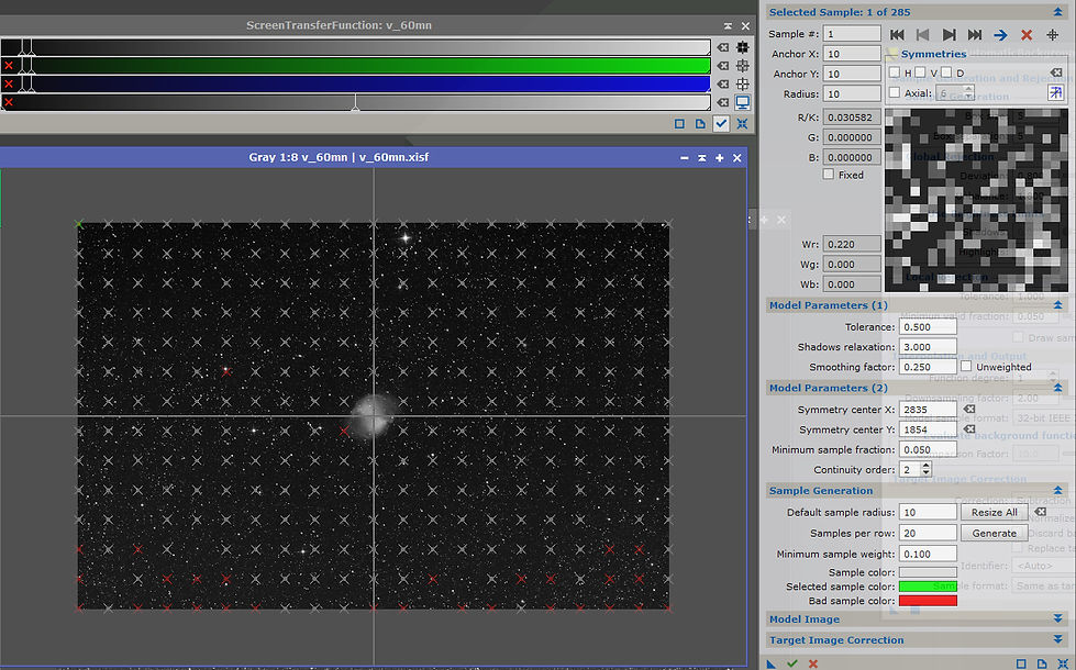
By opening the DBE process on an image, a reticle appears on it: this is the center of the light pollution gradient or any other gradient present in the image that we want to remove. If the gradient is not centered on the image, it is possible to move this center, where the x and Y axes independently by clicking / dragging with the mouse. By clicking on the "Reset" button of the process, the reticle returns to its default position in the center of the image.

DynamicBackgroundExtraction works by generating an image of the gradient corresponding to sample points placed on the target image. These samples must be placed only on the sky background and therefore must not include stars, nebulosities, galaxies, etc.

In order for the generated image to be an accurate representation of the gradients of the target image, the process must have sufficient sample points placed at sufficiently regular intervals.

Sample points can be placed manually anywhere along the image by simply clicking on the target image, or automatically by setting parameters for their placement.

They are represented by squares in the image which can be selected once placed, then possibly moved (mouse) or deleted (DEL key) .

Depending on the relative size of the image, it may be useful to have larger or smaller sample points. By default, the sample point size is set to a radius of 5 pixels, which is too small for most image sizes these days.

A sample size of 10 to 20 is suitable in most cases and depends mainly on the density of the star field and / or nebulosity. Indeed the samples must include the largest portion of the sky (background) possible without however including stars or pieces of objects.

It is possible to modify the size of the samples already placed by entering a new value (default sample radius) and clicking on the "Resize all" button.

Placement of samples can be facilitated by their automatic placement by the process: by clicking on the process reset button once the approximately correct size of the sample points has been determined to remove the manually placed points, then re-entering the radius of the samples. points and clicking on the "Generate" button, which will automatically place samples over the entire image.

To reduce or increase the number of automatically placed samples, just enter a smaller or larger value of "Samples per row" and click again on "Generate". This will have the effect of tightening or spreading the stitches by decreasing or increasing their number per row.

Depending on the content of the image, you can opt for manual or automatic placement. Images that have one or a few prominent objects separated by an empty sky background will often work very well with automatic sample placement (images of galaxies far away from the Milky Way, or small objects that often have a sky background empty around them, like the M27 nebula for example).

For other images, such as those of large nebulae filling the entire field, a manual sample placement approach is usually preferable.

Ancre 7

Case of automatic placement of samples

In this image (Green filter stack) presenting a light pollution gradient, the sample size allowing to occupy good portions of the sky background while passing between the very many stars is 10 (default sample radius) as shown the image below (a larger size would make it very difficult to find a starless zone in the sampling squares ...). One chooses, by increasing for example from 5 to 5 from the initial setting of 5, the largest possible size allowing this.

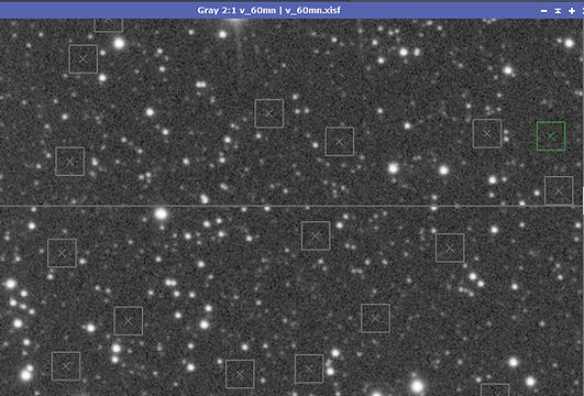
In order to obtain a good image of the gradient we opt for 20 samples per row (samples per row) then click on the Generate button without touching the other parameters.

We note that a large number of areas of the image are not sampled during the automatic generation, only a central band is partially sampled as shown in the image above (brightness of STF decreased to better see the samples ).

These areas are rejected by DynamicBackgroundExtraction in terms of sample weight and defined tolerance, parameters that we will act on to help the process place more sample points automatically.

The default Minimum sample weight setting of 0.750 may work fine in some cases, but here a setting of 0.100 is preferable to automatically place sample points. To change this parameter, we need to click on the Generate button to place the sample points again. The following 3 images show the increasing number of samples automatically placed at 0.5, 0.250 then 0.1 of Minimum sample weight.

We see with the adjustment of this parameter to 0.1 that we are still missing some sampling points and that some are placed but rejected (red). This means that these sample points will not be included in the generation of the model image, which is not desirable.

Indeed even reducing the minimum sampling weight to zero, with the default tolerance of 0.5 and shadows relaxation of 3, some parts of the sky background may still not be sampled. In this case we keep the satisfactory value of 0.1 from which there is no further gain to go down and we adjust the other parameters (tolerance in the case of the weakest zones. brighter, and shadows relaxation in the case of darker areas, not sampled automatically).

The key parameter to adjust now is therefore the tolerance. The default value of 0.500 is generally excellent, but for more intense gradients like the one shown here, you need to increase the tolerance to a larger value.

Values from 1.000 to around 1.500 generally work well, the goal being to set this parameter to the lowest possible value (but not below 0.500) while making sure that all sample points are accepted and that they all lie on the background areas of the image.

In fact, too great a tolerance will have the effect of including stars or bright areas of the object in the sampling, which is obviously not desirable for good modeling of the sky background.

For this image, the tolerance will have to be increased to 1 so as not to have any more unsampled areas. As shown in the following image, the points cover the entire image except the nebula, which is precisely what we are looking for, with a satisfactory number of points.

We note however that if the adjustment of the tolerance parameter made it possible to cover the whole image with the samples, and to make valid some samples which were rejected in the previous step, there are nevertheless some invalid points (red on the picture). At this stage, it will not act to increase the tolerance again to include these points, but rather to go and check by zooming in on the image what is happening at these points.

We will then very often see that these points are placed on stars, or in the halo of large stars, or on a small galaxy or the extensions of an object etc ... and it will then be a matter of simply moving them manually by clicking on them and dragging them to the nearest area including only sky background.

We are now at the stage of the rather tedious procedure of examining each sampling point placed and of moving or removing those which pose a problem even though they may have been validated (not red) by the process. Indeed the sampling points do not need to be perfectly aligned with respect to each other in nice rows as the process has automatically placed them. They just need to sample the image well and only the background. Therefore, do not hesitate to move each sample point slightly relative to the place where it was placed automatically in case a small star is included there, or the fine extensions of the object for example.

It is then useful to zoom in a bit and scan line by line.

The Smoothing factor parameter will take care of smoothing the generated image in order to eliminate the last outliers and to subtract from the target image a model of smoothed background gradients. The default of 0.250 works exceptionally well in almost all cases. You can try lowering it slightly to get a more focused subtraction, but in general values below 0.100 don't work very well because the sample points are taken too literally.

It can also be practical to use the process window to review the samples: the window being displayed in negative, the white corresponds to the sky background, with its noise, and the black area corresponds to an area that is too bright ( a star here) that the sample point overlaps. By dragging the sample point slightly left / right or up / down to place it on the pure background, the problem goes away. You can quickly review all the samples using the left / right arrows located above this window and the sample currently selected appears in green on the image, which allows you to quickly locate it to move it. or delete it if necessary.

If you are not 100% sure that a sample point is actually overlapping a low cloudiness, it is better to move it away from the object in question, or remove it altogether, rather than risk keeping it. . To delete sample points, simply click to select them and press the DEL key on your keyboard. The next sampling point is then selected.

In addition, it is preferable to remove problematic sampling points in the event that too much displacement is required to place it outside the area where it was located, and the surrounding areas are already covered by other dots. 'sampling.

Keep in mind, however, that the smoothing performed on the generated image before the subtraction eliminates some of these outliers.

While you make sure that all sample points are properly placed and do not overlap objects, you can manually add more sample points as well. Sample points added manually by clicking on the target image can also be moved or deleted in the same way.

If, while manipulating the sample points, you find that you want to increase or decrease their size, just enter a new value under Default sample radius. This time however, to avoid erasing all the tedious work you have been doing, don't click the Generate button, as the automatic placement will happen again. Instead, click the Resize all button and this will keep the placement of the sample points, but just resize them.

The Resize all button can also be used to apply other settings such as new tolerance values. This is useful if you suddenly realize that you want to adjust the tolerance but don't want to start all over.

On this image, all the sample points have been checked and the process is therefore ready to be applied to the image.

Some were moved and others deleted due to the presence of small stars, halos of bright stars, or extensions of the nebula.

Adjusting the correction (subtraction or division) is important depending on what you are trying to do. This setting will be discussed in the following sections depending on the application. Here we will use the subtraction function given the nature of the gradient present (subtraction of the light pollution signal).

The gradient map generated is coherent and the image obtained is perfectly corrected for its gradient.

Here we have applied the process to a monochrome image made using poses with a green filter. If the images of the other filters have the same alignment and previous crop, the stars will therefore be in precisely the same place and we will be able to keep the samples of this image to apply the process to the other stacks without having to start all over.

To do this, given that DBE is a dynamic process, closing the window does not allow its parameters to be kept and it will therefore be necessary to create a process icon. This operation is carried out as for all other PixInsight processes: drag the new instance button (blue triangle) of DBE onto the PixInsight workspace.

You can then close the process window because by double-clicking on this process icon the sample points as they were recorded will again be visible on the next selected image.

Finally, it happens that a single gradient extraction is insufficient for some images. There may be more complex gradients which cannot be modeled in a single pass, or a vignetting residue which appears after extracting a gradient etc ...

Performing multiple runs of DBE is a valid option, and sometimes necessary, especially with images that have a lot of sky backgrounds (galaxies and clusters) where small gradients are often very noticeable after the initial extraction.

When performing secondary extractions, you will often find that you will need to readjust the Shadows relaxation and tolerance parameters, and perhaps use smaller samples if small gradients are revealed.

Ancre 6

Case of manual placement of samples

Manual placement of samples is necessary when you need to work with images with complex gradient modeling such as images of large parts or entire molecular clouds, regions filled with IFNs, galaxies with large, small halos. luminous, large emission nebulae covering the entire field ... etc.

Manual sampling is usually necessary when the image is so rich in content that very little can be sampled to properly identify the gradient without sacrificing the true structure of the object. It uses the same parameters and generally follows the same rules as automatic sampling with the essential difference that there is total control on each sample placed.

On this stack Oiii the gradient is clearly visible. Even very narrow band Oiii filters (3.5 nm here) are very sensitive to light pollution and the image is very affected in terms of contrast.

In the presence of this complex case of image with nebulosities over the entire otherwise star-rich field, it is particularly appropriate to use DBE rather than ABE and to proceed to a manual selection of the samples.

To help us with the placement of the points we will use the halpha stack as a reference for the few sky background areas present on the image.

Let us thus locate the zones where there is supposed to be no OIII signal (dark nebulae) and apply the samples accordingly on our image. We can possibly use a boosted STF on the halpha stack to see more clearly in some cases.

We find that for all the added points to be valid, the shadows relaxation parameter has been adjusted to 4.25 because the points placed on the darker areas were not accepted. A sample radius of 25 was chosen, allowing good portions of the sky to be covered without encroaching on the stars in this image.

As in the previous case of automatic sample generation, it was not necessary to act on the tolerance and minimum sample weight parameters.

At each step of adding points, the modeling was evaluated to check its consistency, which is undoubtedly in this type of complex case the most important part of a good extraction. Indeed, a good extraction should ideally identify the gradient and only the gradient. Modeling aspects of your image that are not representative of the gradient would result in a reduction of the object's signal or a loss of certain types of signals, which should be absolutely avoided, especially on an Oiii layer which does not is not the one with the strongest signal!

In images with a lot of sky background like the previous example, erroneous gradient modeling can usually be corrected by simply moving a few samples while in more complex images like this with manual placement, correcting a modeling erroneous may require a much more careful effort.

To evaluate the gradient modeled by DBE, set the Correction option in the Target image correction panel to None, then apply to image.

The map obtained here is completely consistent with what we could observe on the starting image. The darkest and brightest areas absolutely do not correspond to the quantity of Oiii signal present on the different areas of the image, but rather to a modeling of the gradient, which is precisely our objective.

So let's apply the extraction by subtraction and observe the result.

Obviously the image has gained in contrast (visually only by STF of the two images allowing a good comparison of the result). The gradient is much less visible, however there is still a slight noticeable darkening of the lower and upper left corners.

We are therefore going to carry out a 2nd extraction in order to try to overcome this residual gradient, partly due to the difficulty in placing enough points on the image, in particular in these corners supposed to be potentially occupied by the signal.

The Oiii signal and the Hii signal not being at the same location, it is difficult to assess the real presence or not of the Oiii signal from the inspection of the Hii image. On the other hand, one can quite know where one is on that there should not be there, and the first extraction also made it possible to reveal additional zones useful for the sampling.

We create a process icon from the new instance of DBE icon dragged onto the workspace, we close the process, then we open it by clicking on the process icon after selecting the newly created image after the 1st past. The previously created points are thus placed directly on the new image and we only have to add more if possible.

We find that the shadows relaxation parameter had to be further increased to 6 to accept the previously created samples. Note also the increase in the smoothing of the gradient image by increasing the Smoothing factor to 1 to balance the weights of each sample, which can be recommended in this type of complex image case.

Some samples have been added and we obtain the following map, slightly different from the previous one and representative of the residual gradient.

After checking the consistency of this image, we therefore apply the process a second time by subtraction.

On STF visualization, the image obtained further gained in contrast and the gradient was indeed extracted. We can consider at this stage that the image is ready for further processing, and we can save this process icon which may be useful for gradient removal on the Sii layer.

The comparison before / after extraction:

Finally, here is a comparison between the result obtained with two passes of the ABE process on the left and our image resulting from the two passes of DBE on the right.

At first glance the difference is not obvious, yet the signal was clearly altered by the ABE process which considered the differences in brightness of the Oiii signal in the image as significant of a gradient. The result is an enhancement of the less luminous areas and a reduction of the brighter areas, in terms of the Oiii signal in the nebula. This results in a loss of contrast in addition to the irreparable alteration of the gas presence data. The ABE process had been set here to minimize these effects but in some cases it could be much more obvious

Ancre 5

OTHER EXAMPLES OF COMPLEX GRADIENT WITHDRAWALS

Here are two more examples of relatively complex gradients.

Examples of vignetting correction in the absence of flats (valid for vignetting but not dust ...), using the symmetry functions will be added later in this article.

Field of galaxies and stars with complex gradient

This stack of a Luminance seems at first glance to present a simple gradient of the light pollution type, from the lower left corner to the upper right corner.

Let us first try the ABE process, with its basic settings, function degree 1, and a correction by subtraction.

We get the following gradient map which seems to match what the image shows and apply the process.

The result obtained is not satisfactory, a circular gradient has appeared, the sky background is not homogeneous. It is possible that this circular gradient was a poorly corrected vignetting residue which was hidden by the more intense gradient of light pollution and which would have been revealed by the removal of this simple gradient.

Let us try the same process with this time a degree of polynomial function at 4, in case ABE could solve this gradient seeming more complex than at the beginning by developing a more precise gradient map.

The following map is obtained, it is as expected more precise and less linear than the previous one, let's try to apply the process.

The result is worse. ABE is not able to solve this type of gradient, even after several attempts by adjusting other parameters.

Let's move on to the DBE process : we define a sample radius of 20, 10 samples per column, and a correction mode by subtraction. Here you have to adjust the tolerance to 1.65 so that valid samples are placed over the whole image.

After making sure that no sample is placed on a star or galaxy, we start the process.

The result obtained is clearly better but not satisfactory. Indeed dark areas have appeared around galaxies and large stars, as well as a residue of a brighter area in the center between the left galaxy and the center of the image.

This time, let's try a DBE with 25 samples per column, the tolerance still at 1.6, the subtraction mode, and taking care that no sample is in the halo of a large star or in the extensions / halo of galaxies as shown in the following image.

Let's apply the process.

The result obtained is very satisfactory since there remains no trace of gradient, nor of darkened or too bright zones. The sky background is perfectly homogeneous.

This example shows us the power of DBE and the importance that the samples are not placed in the object's halo or near large stars, including their possible halo.

Note also the utility of a large number of samples (475) to solve this type of complex gradient. Let us try all the same to verify this point a test where only 25 samples are used, placed randomly at the 4 corners and in the image, while respecting the previous recommendations of avoidance of galaxies, stars and halos.

The extraction is incomplete since this brighter zone remains in the center of the image.

It is therefore a question of using a sufficiently large number of samples, which however increases the work necessary to verify them all once they are generated and placed by the process (verify the absence of a small star in the sample and keep them away from large stars and object halos while maintaining the fullest presence of samples throughout the field.).

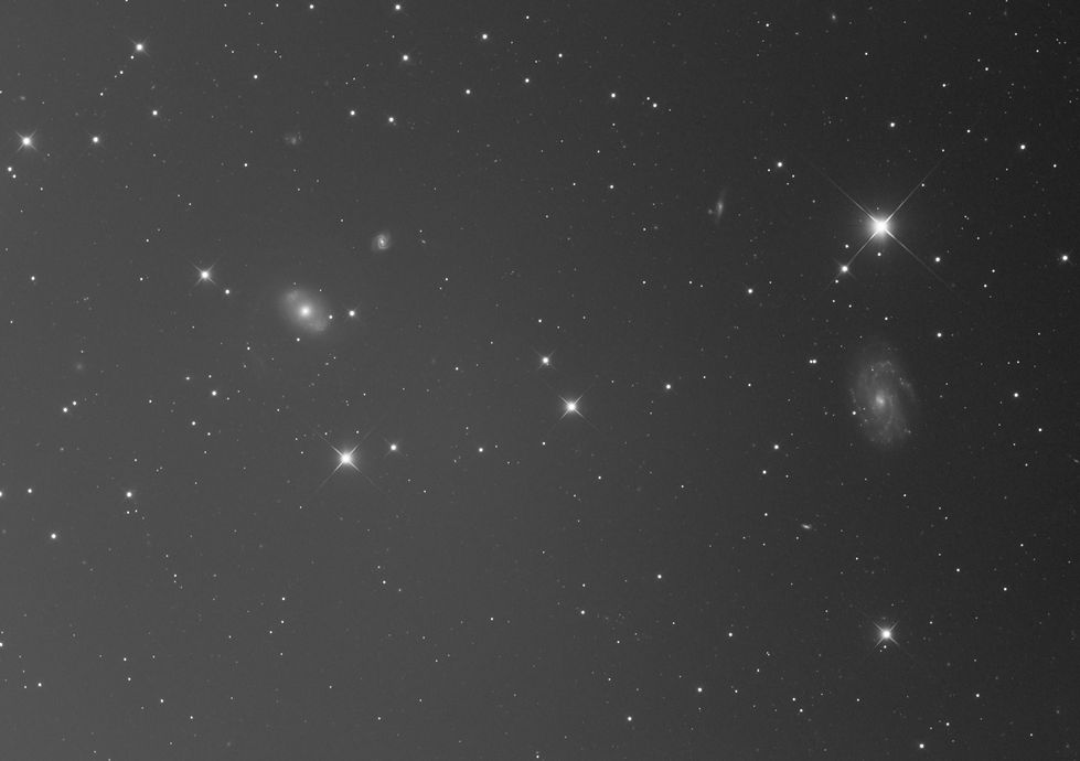
Galaxy occupying a large part of the field and presence of IFN

I am a paragraph. Click here to add your own text and edit me. It's easy.

This image (Luminance stack) presents a slight gradient, but still clearly visible with the STF.

A boosted STF will confirm the existence of a residue of vignetting probably mixed with a left-right gradient of light pollution.

Let's try the ABE process with a degree of polynomial function of 2, in subtraction mode:

As in the previous example, the result is not satisfactory with ABE since we obtain an important darkening around the galaxy, typical of gradient withdrawals failed on galaxy images.

Indeed it is very likely that the process takes the brilliant heart of the galaxy, then its less luminous extensions, then the dark sky background as a decline in luminosity from the center to the edges of the image, namely a vignetting. By applying a correction model for this vignetting, we end up with a periphery of the image brighter than the center, except for the galaxy which, due to its high starting luminosity, remains very bright. The result is then typically this black rim around the object.

Let us observe the behavior of ABE with a degree of polynomial function of 1:

the generated map shows the detection by ABE of a gradient from the bottom left to the top right but the darkening of the other two corners is not taken into account and the correction is not complete as shown by the boosted STF above , which will inevitably be problematic during subsequent treatments, all the more so in this case of the presence of very weak IFN nebulosities in the sky background.

So let's move on to the DBE process: the sample size chosen is 25 with 25 samples per column, and the tolerance and relaxation shadows parameters are adjusted so that the samples cover the entire field except the galaxy.

Each sample is then visually checked to ensure that it does not contain a small star, and those closest to the galaxy's halo and large star halos are discarded or removed. Care is also taken not to place dots on the small irregular galaxy and weak IFN nebulosities by increasing the contrast by adjusting the STF.

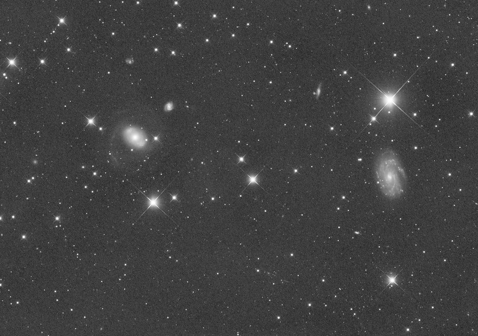
After checking the card obtained, the process is applied.

Gradient removal is performed perfectly, without darkening around the galaxy or the big stars, as confirmed by the image below with boosted STF.

To come: examples of gradient extraction due to the absence of flats or to a very poor correction of vignetting (overcorrection, under-correction ...) using the Division function and the advanced symmetry functions.

Top of page